Otto Cycle - Principles and Calculations

Graham
Garcia

The Otto cycle is best exemplified by the sparkplug engine. Regularly seen in car engines and lawnmowers, this cycle is versatile in the different jobs it can do as well as the ability to be made bigger or smaller with relative ease. In this article, you will learn the principles behind the Otto cycle, calculations, and applications.

Principles of the Otto Cycle

The Otto cycle is one of the most commonly seen cycles. Because of its simplicity and ability to expand to multiple cycles running simultaneously, it is one of the most versatile thermodynamic cycles. The cycle runs off of gasoline to produce mechanical work output.

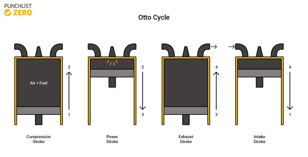
The cycle starts when the fuel initially enters into the cycle at step one. The fuel mixes with air to induce combustion into the closed system. Next, the mixture runs through a compression stroke. The mixture compresses and allows the piston to move into a position to produce power. Igniting the compressed mixture in a power stroke extracts energy through the piston. Lastly, the exhaust stroke occurs, eliminating all burnt-up fuel fumes. The cycle simply repeats itself by introducing air

Calculations of the Otto Cycle

Since the Otto cycle uses air and fuel as the working fluids of the system it is standard to use air values to help analyze the cycle. Unlike most cycles where tracking of enthalpy occurs throughout the analysis, the Otto cycle mainly tracks the temperatures and specific volumes at each state to find the true values.

State 1 ➔ 2 (Compression Stroke)

To first analyze the compression stroke of the Otto cycle few values require definition. Temperature(T1) at state one typically provides a known quantity, usually around room temperature of 290-300 K. Observers usually also know compression ratio(Cr). The Cr of the Otto Cycle registers significantly lower than that of a diesel cycle.

First use the Temperature at state one and air tables to define the internal energy(u1), the relative pressure(Pr1), and the relative volume(Vr1).

The compression ratio and the relative volume allow the determination of the relative volume(Vr2) of state 2.

$C_r = \frac{V_1}{V_2} = \frac{v_{r1}}{v_{r2}}$

This equation may be simplified into a more useable form.

$v_{r2} = \frac{v_{r1}}{C_r}$

The found relative volume and air tables allow for the determination of temperature(T2), relative pressure(Pr2), and internal energy(u2).

State 2 ➔ 3 (Power Stroke)

Before working on this stage, the desired temperature after the power stroke requires determination(T3). The power stroke is an isochoric process, meaning that while pressure(P2➔P3) and temperature(T2➔T3) change the volume(V2=V3) stays the same. Heat added during this process occurs by using the specific heat at constant volume(Cv).

$q_{in} = C_v(T_3 - T_2)$

Also, by using the third stage temperature and the air tables, the relative volume(Vr3), relative pressure(Pr3), and internal energy(u3) can be found.

State 3 ➔ 4 (Exhaust Stroke)

The compression ratio and the found relative volume at stage 3, allow for determination of the relative volume(Vr4) at stage 4.

$C_r = \frac{v_{r4}}{v_{r3}}$

This equation may be simplified into a more useable form.

$v_{r4} = C_r v_{r3}$

The found value and the air tables allow for the calculation of the temperature(T4), internal energy(u4), and relative pressure(Pr4).

State 4 ➔ 1 (Intake Stroke)

Since all the intermediate values are now found the last part is to analyze the Otto cycle as a whole. First, find the mass of the air in the system using the ideal gas law.

$m = \frac{P_1 v_1}{R T_1}$

Next using the found mass, calculate the heat in and out of the system.

$Q_{in} = m(u_3 - u_2)$

$Q_{out} = m(u_4 - u_1)$

Then, determination of net work may occur.

$W_{net} = Q_{in} - Q_{out}$

Finally, these values determine the thermal efficiency and mean effective pressure of the Otto cycle.

$\eta_{thermal} = \frac{W_{net}}{Q_{in}}$

$MEP = \frac{W_{net}}{v_1 - v_2}$

$MEP = \frac{W_{net}}{v_1(1 - \frac{1}{C_r})}$

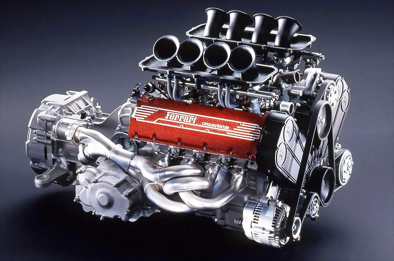
Applicable Uses of the Otto Cycle

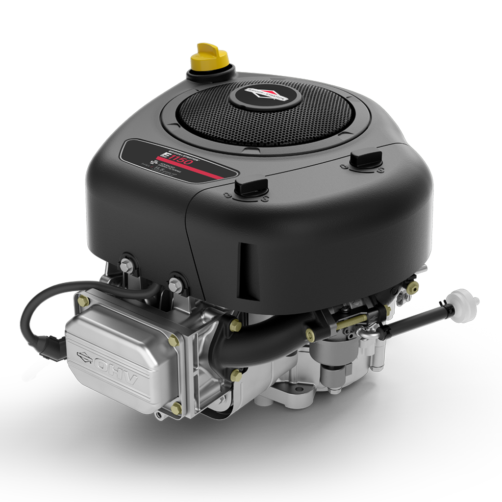
Riding Lawn Mower Engines | Briggs & Stratton — *COURTESY: BRIGGS AND STRATTON*

The Otto cycle provide a large amount of useful applications in real life. It is the most compact and versatile thermodynamic cycle of the bunch. Running at the most base version using only one cylinder, it powers small machines and generators. It is used in lawnmowers, smaller industrial pumps and compressors, cars, and many other different machines. One of the reasons for its ubiquity is its ability to scale to larger systems. Cars are able to pack 4-12 concurrent and connected cylinders that perform the Otto cycle to generate massive amounts of power using a relatively small amount of fuel.

Otto Cycle – Principles and Calculations

Engineering

Principles of the Otto Cycle